KBMOD Visualization#
This notebook demonstrates the basic functionality for working with RawImages and visualizing them.
Setup kbmod visualization demo#
Before importing, make sure you have installed kbmod using pip install . in the root directory. Also be sure you are running with python3 and using the correct notebook kernel.
[1]:
# everything we will need for this demo
import kbmod.search as kb
import matplotlib.pyplot as plt
import math
import numpy as np
import os

im_path = "../data/small/"
res_path = "./results"
Loading data for visualization demo#
A. Load a file for visualization:#
The layered_image is loaded given the path and filename to the FITS file as well as the PSF for the image. We use a default psf.
[2]:
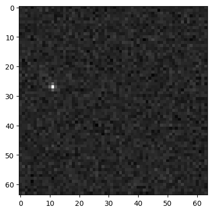
p = kb.psf(1.0)
im = kb.layered_image(im_path + "000000.fits", p)
print(f"Loaded a {im.get_width()} by {im.get_height()} image at time {im.get_time()}")
Loaded a 64 by 64 image at time 57130.19921875
We can visualize the image using matplotlib.
Note: The data/demo images contain a single bright object, so the majority of the image should be empty with a single bright spot.
[3]:
plt.imshow(im.get_science(), cmap="gray")
[3]:
<matplotlib.image.AxesImage at 0x7fc53e417ac0>
B. Load a stack of images#
A load collection of layered_images at different times.
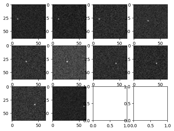
[4]:
files = [im_path + f for f in os.listdir(im_path) if ".fits" in f]
files.sort()

# Create default PSFs for each image.
all_psfs = [p for _ in range(len(files))]

# Load the images.
stack = kb.image_stack(files, all_psfs)

num_images = stack.img_count()
print(f"Loaded {num_images} images.")
.Loaded 10 images.
.........
Display each image.
[5]:
w = 4
h = math.ceil(num_images / w)

fig, axs = plt.subplots(h, w)
for i in range(h):
    for j in range(w):
        ind = w * i + j
        if ind < num_images:
            axs[i, j].imshow(stack.get_single_image(ind).get_science(), cmap="gray")
Create stamps#
We use two objects to create stamps: * search_stack - provides the machinery for making predictions on the image (needed to handle the various corrections). * trajectory - Contains the information about where to place the stamps (the underlying trajectory).
[6]:
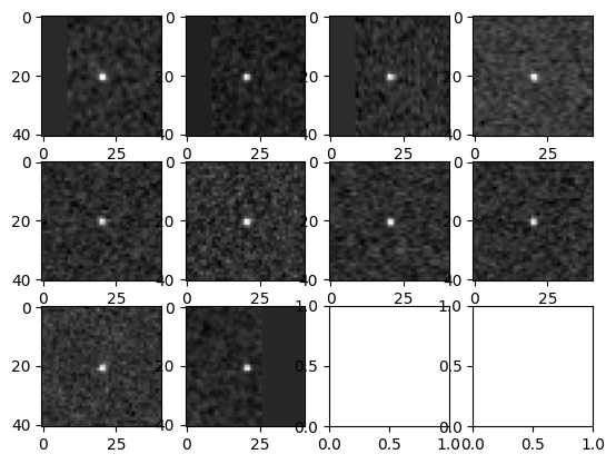
# Create the trajectory with a given parameters and then the trajectory result.
trj = kb.trajectory()
trj.x = 11
trj.y = 27
trj.x_v = 16.0
trj.y_v = 3.3

# Create the search stack.
search = kb.stack_search(stack)

# Create the stamps around this trajectory.
stamps = search.science_viz_stamps(trj, 20)
Now we can display the stamps around each predicted object position.
[7]:
fig, axs = plt.subplots(h, w)
for i in range(h):
    for j in range(w):
        ind = w * i + j
        if ind < num_images:
            axs[i, j].imshow(stamps[ind], cmap="gray")
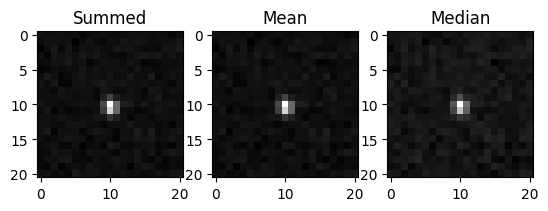
We can also compute the sum, mean, or median stamp. The stamp functions take a list of bools corresponding to whether each time is valid. These can be extracted from the result data. You can use an empty array (as we do below) to build the stamp out of all valid times.
[8]:
fig, axs = plt.subplots(1, 3)

axs[0].imshow(search.summed_sci_stamp(trj, 10, []), cmap="gray")
axs[0].set_title("Summed")

axs[1].imshow(search.mean_sci_stamp(trj, 10, []), cmap="gray")
axs[1].set_title("Mean")

axs[2].imshow(search.median_sci_stamp(trj, 10, []), cmap="gray")
axs[2].set_title("Median")
[8]:
Text(0.5, 1.0, 'Median')
[ ]: